Jak dodać napis ggplot2 o innym rozmiarze i kolorze?
Używam ggplot2, aby poprawić opady.
Oto powtarzalny przykład tego, co chcę osiągnąć:
library(ggplot2)
library(gridExtra)
secu <- seq(1, 16, by=2)
melt.d <- data.frame(y=secu, x=LETTERS[1:8])
m <- ggplot(melt.d, aes(x=x, y=y)) +
  geom_bar(fill="darkblue") +
  labs(x="Weather    stations", y="Accumulated Rainfall [mm]") +
  opts(axis.text.x=theme_text(angle=-45, hjust=0, vjust=1),
       title=expression("Rainfall"), plot.margin = unit(c(1.5, 1, 1, 1), "cm"),
       plot.title = theme_text(size = 25, face = "bold", colour = "black", vjust = 5))
z <- arrangeGrob(m, sub = textGrob("Location", x = 0, hjust = -3.5, vjust = -33, gp = gpar(fontsize = 18, col = "gray40"))) #Or guessing x and y with just option
z
Nie wiem jak uniknąć używania liczb zgadywania na hjust i vjust na ggplot2? Czy istnieje lepszy sposób na umieszczenie napisów (nie tylko za pomocą \n, ale napisów o innym kolorze i rozmiarze tekstu)?
Muszę mieć możliwość korzystania z ggsave, aby mieć plik pdf.
Oto dwa powiązane pytania:
Dodaj przypis poza obszarem działki w R?
Jak dodać podtytuł i zmienić rozmiar czcionki działek ggplot w R?
Dzięki za pomoc.7 answers
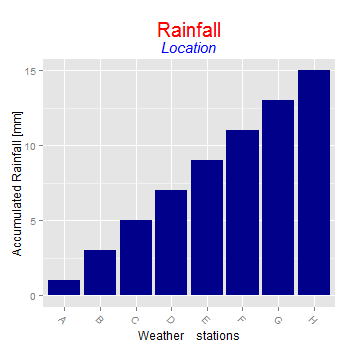
2.1.0.9000 lub nowsze) mają napisy i napisy poniżej jako wbudowane funkcje. Oznacza to, że możesz to zrobić:
library(ggplot2) # 2.1.0.9000+

secu <- seq(1, 16, by=2)
melt.d <- data.frame(y=secu, x=LETTERS[1:8])

m <-  ggplot(melt.d, aes(x=x, y=y))
m <- m + geom_bar(fill="darkblue", stat="identity")
m <- m + labs(x="Weather    stations",
              y="Accumulated Rainfall [mm]",
              title="Rainfall",
              subtitle="Location")
m <- m + theme(axis.text.x=element_text(angle=-45, hjust=0, vjust=1))
m <- m + theme(plot.title=element_text(size=25, hjust=0.5, face="bold", colour="maroon", vjust=-1))
m <- m + theme(plot.subtitle=element_text(size=18, hjust=0.5, face="italic", color="black"))
m
Warning: date(): Invalid date.timezone value 'Europe/Kyiv', we selected the timezone 'UTC' for now. in /var/www/agent_stack/data/www/doraprojects.net/template/agent.layouts/content.php on line 54
2017-07-12 09:15:10
Ignoruj tę odpowiedź ggplot2 Wersja 2.2.0 posiada funkcje tytułu i napisów. Zobacz odpowiedź @ hrbrmstr poniżej .
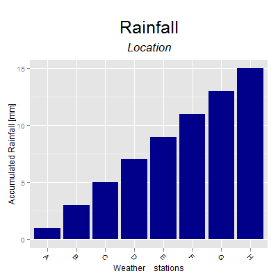
Możesz użyć zagnieżdżonych funkcji atop wewnątrz expression, aby uzyskać różne rozmiary.
EDIT zaktualizowany kod dla ggplot2 0.9.3
m <-  ggplot(melt.d, aes(x=x, y=y)) +
     geom_bar(fill="darkblue", stat = "identity") +
     labs(x="Weather    stations", y="Accumulated Rainfall [mm]") +
     ggtitle(expression(atop("Rainfall", atop(italic("Location"), "")))) +
     theme(axis.text.x = element_text(angle=-45, hjust=0, vjust=1),
     #plot.margin = unit(c(1.5, 1, 1, 1), "cm"),
     plot.title = element_text(size = 25, face = "bold", colour = "black", vjust = -1))
Warning: date(): Invalid date.timezone value 'Europe/Kyiv', we selected the timezone 'UTC' for now. in /var/www/agent_stack/data/www/doraprojects.net/template/agent.layouts/content.php on line 54
2017-07-12 04:59:16
Wygląda na to, że opts jest przestarzały od ggplot 2 0.9.1 i nie działa. To działało dla mnie z najnowszymi wersjami od Dziś: + ggtitle(expression(atop("Top line", atop(italic("2nd line"), "")))).
Warning: date(): Invalid date.timezone value 'Europe/Kyiv', we selected the timezone 'UTC' for now. in /var/www/agent_stack/data/www/doraprojects.net/template/agent.layouts/content.php on line 54
2013-02-03 01:42:46
Ta wersja używa funkcji gtable. Pozwala na dwa wiersze tekstu w tytule. Tekst, rozmiar, kolor i powierzchnia czcionki każdej linii można ustawić niezależnie od drugiej. Jednak funkcja zmodyfikuje Wykres tylko za pomocą jednego panelu wykresu.
Minor edit: Aktualizacja do ggplot2 v2.0.0
# The original plot
library(ggplot2)

secu <- seq(1, 16, by = 2)
melt.d <- data.frame(y = secu, x = LETTERS[1:8])

m <- ggplot(melt.d, aes(x = x, y = y)) +
     geom_bar(fill="darkblue", stat = "identity") +
     labs(x = "Weather    stations", y = "Accumulated Rainfall [mm]") +
     theme(axis.text.x = element_text(angle = -45, hjust = 0, vjust = 1))


# The function to set text, size, colour, and face
plot.title = function(plot = NULL, text.1 = NULL, text.2 = NULL,
   size.1 = 12,  size.2 = 12,
   col.1 = "black", col.2 = "black",
   face.1 = "plain",  face.2 = "plain") {

library(gtable)
library(grid)

gt = ggplotGrob(plot)

text.grob1 = textGrob(text.1, y = unit(.45, "npc"),
   gp = gpar(fontsize = size.1, col = col.1, fontface = face.1))
text.grob2 = textGrob(text.2,  y = unit(.65, "npc"),
   gp = gpar(fontsize = size.2, col = col.2, fontface = face.2))

text = matrix(list(text.grob1, text.grob2), nrow = 2)
text = gtable_matrix(name = "title", grobs = text,
   widths = unit(1, "null"),
   heights = unit.c(unit(1.1, "grobheight", text.grob1) + unit(0.5, "lines"), unit(1.1,  "grobheight", text.grob2) + unit(0.5, "lines")))

gt = gtable_add_grob(gt, text, t = 2, l = 4)
gt$heights[2] = sum(text$heights)

class(gt) =  c("Title", class(gt))

gt
}

# A print method for the plot
print.Title <- function(x) {
   grid.newpage()
   grid.draw(x)
}


# Try it out - modify the original plot
p = plot.title(m, "Rainfall", "Location",
   size.1 = 20, size.2 = 15,
   col.1 = "red", col.2 = "blue",
   face.2 = "italic")

p
Warning: date(): Invalid date.timezone value 'Europe/Kyiv', we selected the timezone 'UTC' for now. in /var/www/agent_stack/data/www/doraprojects.net/template/agent.layouts/content.php on line 54
2016-08-01 03:11:19
Nie jest zbyt trudno dodać grobs do gtable i zrobić w ten sposób wymyślny tytuł,
library(ggplot2)
library(grid)
library(gridExtra)
library(magrittr)
library(gtable)

p <- ggplot() +
  theme(plot.margin = unit(c(0.5, 1, 1, 1), "cm"))

lg <- list(textGrob("Rainfall", x=0, hjust=0,
                    gp = gpar(fontsize=24, fontfamily="Skia", face=2, col="turquoise4")),
               textGrob("location", x=0, hjust=0,
                        gp = gpar(fontsize=14, fontfamily="Zapfino", fontface=3, col="violetred1")),
           pointsGrob(pch=21, gp=gpar(col=NA, cex=0.5,fill="steelblue")))

margin <- unit(0.2, "line")
tg <- arrangeGrob(grobs=lg, layout_matrix=matrix(c(1,2,3,3), ncol=2),
                  widths = unit.c(grobWidth(lg[[1]]), unit(1,"null")),
                  heights = do.call(unit.c, lapply(lg[c(1,2)], grobHeight)) + margin)

grid.newpage()
ggplotGrob(p) %>%
  gtable_add_rows(sum(tg$heights), 0) %>%
  gtable_add_grob(grobs=tg, t = 1, l = 4)  %>%
  grid.draw()

Warning: date(): Invalid date.timezone value 'Europe/Kyiv', we selected the timezone 'UTC' for now. in /var/www/agent_stack/data/www/doraprojects.net/template/agent.layouts/content.php on line 54
2016-03-16 19:43:54
Możesz użyć zawijania wykresu w siatkę.Uporządkuj i przekaż Niestandardowy tytuł oparty na siatce,

library(ggplot2)
library(gridExtra)

p <- ggplot() +
  theme(plot.margin = unit(c(0.5, 1, 1, 1), "cm"))

tg <- grobTree(textGrob("Rainfall", y=1, vjust=1, gp = gpar(fontsize=25, face=2, col="black")),
               textGrob("location", y=0, vjust=0, gp = gpar(fontsize=12, face=3, col="grey50")),
               cl="titlegrob")
heightDetails.titlegrob <- function(x) do.call(sum,lapply(x$children, grobHeight))

grid.arrange(p, top = tg)
Warning: date(): Invalid date.timezone value 'Europe/Kyiv', we selected the timezone 'UTC' for now. in /var/www/agent_stack/data/www/doraprojects.net/template/agent.layouts/content.php on line 54
2016-02-12 21:40:01
Być może zauważyłeś, że w kodzie Sandy nie ma pogrubionego tytułu dla "Rainfall" - instrukcja, aby to pogrubić, powinna występować w funkcji atop (), a nie w funkcji theme ().
ggplot(melt.d, aes(x=x, y=y)) +
 geom_bar(fill="darkblue", stat = "identity") +
 labs(x="Weather    stations", y="Accumulated Rainfall [mm]") +
 ggtitle(expression(atop(bold("Rainfall"), atop(italic("Location"), "")))) +
 theme(axis.text.x = element_text(angle=-45, hjust=0, vjust=1),
 plot.title = element_text(size = 25, colour = "black", vjust = -1))

Warning: date(): Invalid date.timezone value 'Europe/Kyiv', we selected the timezone 'UTC' for now. in /var/www/agent_stack/data/www/doraprojects.net/template/agent.layouts/content.php on line 54
2015-09-21 01:49:31