Dodaj wspólną legendę dla połączonych ggplotów
Mam dwa ggploty, które wyrównuję poziomo z grid.arrange. Przejrzałem wiele postów na forum, ale wszystko, co próbuję, wydaje się być poleceniami, które są teraz aktualizowane i nazywane czymś innym.
Moje dane wyglądają tak;
# Data plot 1
        axis1     axis2
group1 -0.212201  0.358867
group2 -0.279756 -0.126194
group3  0.186860 -0.203273
group4  0.417117 -0.002592
group1 -0.212201  0.358867
group2 -0.279756 -0.126194
group3  0.186860 -0.203273
group4  0.186860 -0.203273

# Data plot 2
        axis1     axis2
group1  0.211826 -0.306214
group2 -0.072626  0.104988
group3 -0.072626  0.104988
group4 -0.072626  0.104988
group1  0.211826 -0.306214
group2 -0.072626  0.104988
group3 -0.072626  0.104988
group4 -0.072626  0.104988

#And I run this:
library(ggplot2)
library(gridExtra)


groups=c('group1','group2','group3','group4','group1','group2','group3','group4')

x1=data1[,1]
y1=data1[,2]

x2=data2[,1]
y2=data2[,2]

p1=ggplot(data1, aes(x=x1, y=y1,colour=groups)) + geom_point(position=position_jitter(w=0.04,h=0.02),size=1.8)

p2=ggplot(data2, aes(x=x2, y=y2,colour=groups)) + geom_point(position=position_jitter(w=0.04,h=0.02),size=1.8)

#Combine plots
p3=grid.arrange(
p1 + theme(legend.position="none"), p2+ theme(legend.position="none"), nrow=1, widths = unit(c(10.,10), "cm"), heights = unit(rep(8, 1), "cm")))
Jak wyodrębnić legendę z któregokolwiek z tych wątków i dodać ją do dołu / środka połączonego wątku?
7 answers
Aktualizacja 2015-Luty
Zobacz odpowiedź Stevena poniżej
df1 <- read.table(text="group x y
group1 -0.212201 0.358867
group2 -0.279756 -0.126194
group3 0.186860 -0.203273
group4 0.417117 -0.002592
group1 -0.212201 0.358867
group2 -0.279756 -0.126194
group3 0.186860 -0.203273
group4 0.186860 -0.203273",header=TRUE)
df2 <- read.table(text="group x y
group1 0.211826 -0.306214
group2 -0.072626 0.104988
group3 -0.072626 0.104988
group4 -0.072626 0.104988
group1 0.211826 -0.306214
group2 -0.072626 0.104988
group3 -0.072626 0.104988
group4 -0.072626 0.104988",header=TRUE)
library(ggplot2)
library(gridExtra)
p1 <- ggplot(df1, aes(x=x, y=y,colour=group)) + geom_point(position=position_jitter(w=0.04,h=0.02),size=1.8) + theme(legend.position="bottom")
p2 <- ggplot(df2, aes(x=x, y=y,colour=group)) + geom_point(position=position_jitter(w=0.04,h=0.02),size=1.8)
#extract legend
#https://github.com/hadley/ggplot2/wiki/Share-a-legend-between-two-ggplot2-graphs
g_legend<-function(a.gplot){
tmp <- ggplot_gtable(ggplot_build(a.gplot))
leg <- which(sapply(tmp$grobs, function(x) x$name) == "guide-box")
legend <- tmp$grobs[[leg]]
return(legend)}
mylegend<-g_legend(p1)
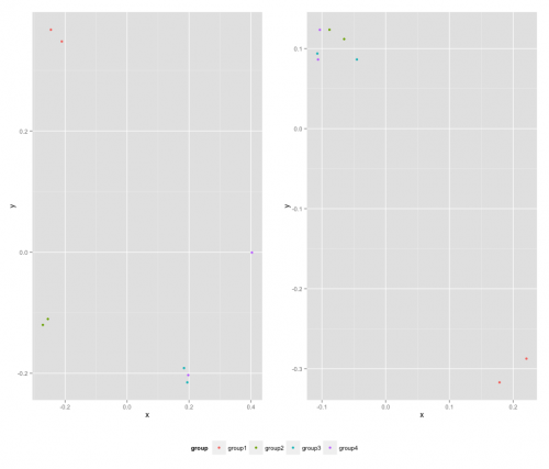
p3 <- grid.arrange(arrangeGrob(p1 + theme(legend.position="none"),
p2 + theme(legend.position="none"),
nrow=1),
mylegend, nrow=2,heights=c(10, 1))
Oto wynikowy Wykres:
Warning: date(): Invalid date.timezone value 'Europe/Kyiv', we selected the timezone 'UTC' for now. in /var/www/agent_stack/data/www/doraprojects.net/template/agent.layouts/content.php on line 54
2017-05-23 12:18:22
Odpowiedź Rolanda wymaga aktualizacji. Zobacz: https://github.com/hadley/ggplot2/wiki/Share-a-legend-between-two-ggplot2-graphs
Ta metoda została zaktualizowana dla ggplot2 v1.0.0.
library(ggplot2)
library(gridExtra)
library(grid)


grid_arrange_shared_legend <- function(...) {
    plots <- list(...)
    g <- ggplotGrob(plots[[1]] + theme(legend.position="bottom"))$grobs
    legend <- g[[which(sapply(g, function(x) x$name) == "guide-box")]]
    lheight <- sum(legend$height)
    grid.arrange(
        do.call(arrangeGrob, lapply(plots, function(x)
            x + theme(legend.position="none"))),
        legend,
        ncol = 1,
        heights = unit.c(unit(1, "npc") - lheight, lheight))
}

dsamp <- diamonds[sample(nrow(diamonds), 1000), ]
p1 <- qplot(carat, price, data=dsamp, colour=clarity)
p2 <- qplot(cut, price, data=dsamp, colour=clarity)
p3 <- qplot(color, price, data=dsamp, colour=clarity)
p4 <- qplot(depth, price, data=dsamp, colour=clarity)
grid_arrange_shared_legend(p1, p2, p3, p4)
Zwróć uwagę na brak ggplot_gtable i ggplot_build. ggplotGrob jest używany zamiast. Ten przykład jest nieco bardziej zawiły niż powyższe rozwiązanie, ale nadal rozwiązał go dla mnie.
Warning: date(): Invalid date.timezone value 'Europe/Kyiv', we selected the timezone 'UTC' for now. in /var/www/agent_stack/data/www/doraprojects.net/template/agent.layouts/content.php on line 54
2016-06-23 11:43:16
Możesz również użyć ggarrangez pakietu ggpubr i ustawić "common.legend = TRUE": {]}
library(ggpubr)

dsamp <- diamonds[sample(nrow(diamonds), 1000), ]
p1 <- qplot(carat, price, data = dsamp, colour = clarity)
p2 <- qplot(cut, price, data = dsamp, colour = clarity)
p3 <- qplot(color, price, data = dsamp, colour = clarity)
p4 <- qplot(depth, price, data = dsamp, colour = clarity)

ggarrange(p1, p2, p3, p4, ncol=2, nrow=2, common.legend = TRUE, legend="bottom")

Warning: date(): Invalid date.timezone value 'Europe/Kyiv', we selected the timezone 'UTC' for now. in /var/www/agent_stack/data/www/doraprojects.net/template/agent.layouts/content.php on line 54
2017-10-29 21:08:33
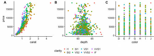
Sugeruję użycie cowplot. Z ich R winieta :
# load cowplot
library(cowplot)

# down-sampled diamonds data set
dsamp <- diamonds[sample(nrow(diamonds), 1000), ]

# Make three plots.
# We set left and right margins to 0 to remove unnecessary spacing in the
# final plot arrangement.
p1 <- qplot(carat, price, data=dsamp, colour=clarity) +
   theme(plot.margin = unit(c(6,0,6,0), "pt"))
p2 <- qplot(depth, price, data=dsamp, colour=clarity) +
   theme(plot.margin = unit(c(6,0,6,0), "pt")) + ylab("")
p3 <- qplot(color, price, data=dsamp, colour=clarity) +
   theme(plot.margin = unit(c(6,0,6,0), "pt")) + ylab("")

# arrange the three plots in a single row
prow <- plot_grid( p1 + theme(legend.position="none"),
           p2 + theme(legend.position="none"),
           p3 + theme(legend.position="none"),
           align = 'vh',
           labels = c("A", "B", "C"),
           hjust = -1,
           nrow = 1
           )

# extract the legend from one of the plots
# (clearly the whole thing only makes sense if all plots
# have the same legend, so we can arbitrarily pick one.)
legend_b <- get_legend(p1 + theme(legend.position="bottom"))

# add the legend underneath the row we made earlier. Give it 10% of the height
# of one plot (via rel_heights).
p <- plot_grid( prow, legend_b, ncol = 1, rel_heights = c(1, .2))
p
Warning: date(): Invalid date.timezone value 'Europe/Kyiv', we selected the timezone 'UTC' for now. in /var/www/agent_stack/data/www/doraprojects.net/template/agent.layouts/content.php on line 54
2017-06-26 18:07:48
@Giuseppe, możesz rozważyć to dla elastycznej specyfikacji układu działek (zmodyfikowany z tutaj):
library(ggplot2)
library(gridExtra)
library(grid)

grid_arrange_shared_legend <- function(..., nrow = 1, ncol = length(list(...)), position = c("bottom", "right")) {

  plots <- list(...)
  position <- match.arg(position)
  g <- ggplotGrob(plots[[1]] + theme(legend.position = position))$grobs
  legend <- g[[which(sapply(g, function(x) x$name) == "guide-box")]]
  lheight <- sum(legend$height)
  lwidth <- sum(legend$width)
  gl <- lapply(plots, function(x) x + theme(legend.position = "none"))
  gl <- c(gl, nrow = nrow, ncol = ncol)

  combined <- switch(position,
                     "bottom" = arrangeGrob(do.call(arrangeGrob, gl),
                                            legend,
                                            ncol = 1,
                                            heights = unit.c(unit(1, "npc") - lheight, lheight)),
                     "right" = arrangeGrob(do.call(arrangeGrob, gl),
                                           legend,
                                           ncol = 2,
                                           widths = unit.c(unit(1, "npc") - lwidth, lwidth)))
  grid.newpage()
  grid.draw(combined)

}
Dodatkowe argumenty nrow i ncol kontrolują układ ułożonych Wykresów:
dsamp <- diamonds[sample(nrow(diamonds), 1000), ]
p1 <- qplot(carat, price, data = dsamp, colour = clarity)
p2 <- qplot(cut, price, data = dsamp, colour = clarity)
p3 <- qplot(color, price, data = dsamp, colour = clarity)
p4 <- qplot(depth, price, data = dsamp, colour = clarity)
grid_arrange_shared_legend(p1, p2, p3, p4, nrow = 1, ncol = 4)
grid_arrange_shared_legend(p1, p2, p3, p4, nrow = 2, ncol = 2)


Warning: date(): Invalid date.timezone value 'Europe/Kyiv', we selected the timezone 'UTC' for now. in /var/www/agent_stack/data/www/doraprojects.net/template/agent.layouts/content.php on line 54
2016-07-18 17:22:44
Jeśli wykreślasz te same zmienne w obu wykresach, najprostszym sposobem byłoby połączenie ramek danych w jedną, a następnie użycie facet_wrap.
Dla Twojego przykładu:
big_df <- rbind(df1,df2)

big_df <- data.frame(big_df,Df = rep(c("df1","df2"),
times=c(nrow(df1),nrow(df2))))

ggplot(big_df,aes(x=x, y=y,colour=group))
+ geom_point(position=position_jitter(w=0.04,h=0.02),size=1.8)
+ facet_wrap(~Df)

Kolejny przykład wykorzystujący zestaw danych diamentów. To pokazuje, że można nawet zrobić to działa, jeśli masz tylko jedną zmienną wspólną między Wykresów.
diamonds_reshaped <- data.frame(price = diamonds$price,
independent.variable = c(diamonds$carat,diamonds$cut,diamonds$color,diamonds$depth),
Clarity = rep(diamonds$clarity,times=4),
Variable.name = rep(c("Carat","Cut","Color","Depth"),each=nrow(diamonds)))

ggplot(diamonds_reshaped,aes(independent.variable,price,colour=Clarity)) +
geom_point(size=2) + facet_wrap(~Variable.name,scales="free_x") +
xlab("")

Jedyną trudną rzeczą w drugim przykładzie jest to, że zmienne czynnika są zmuszane do numeryczne po połączeniu wszystkiego w jedną ramkę danych. Więc idealnie, zrobisz to głównie wtedy, gdy wszystkie interesujące Cię zmienne są tego samego typu.
Warning: date(): Invalid date.timezone value 'Europe/Kyiv', we selected the timezone 'UTC' for now. in /var/www/agent_stack/data/www/doraprojects.net/template/agent.layouts/content.php on line 54
2018-01-17 09:20:32
@ Guiseppe:
Nie mam pojęcia o grobach itp., ale zebrałem rozwiązanie dla dwóch działek, powinno być możliwe rozszerzenie na dowolną liczbę, ale jej nie ma w funkcji sexy:
plots <- list(p1, p2)
g <- ggplotGrob(plots[[1]] + theme(legend.position="bottom"))$grobs
legend <- g[[which(sapply(g, function(x) x$name) == "guide-box")]]
lheight <- sum(legend$height)
tmp <- arrangeGrob(p1 + theme(legend.position = "none"), p2 + theme(legend.position = "none"), layout_matrix = matrix(c(1, 2), nrow = 1))
grid.arrange(tmp, legend, ncol = 1, heights = unit.c(unit(1, "npc") - lheight, lheight))
Warning: date(): Invalid date.timezone value 'Europe/Kyiv', we selected the timezone 'UTC' for now. in /var/www/agent_stack/data/www/doraprojects.net/template/agent.layouts/content.php on line 54
2016-01-16 11:41:05