wyrównanie zdjęć z wykresem w r
Najpierw pomyślałem, że muszę to zrobić ręcznie w powerpoint, potem pomyślałem, że może być spróbuj z R, jeśli istnieje rozwiązanie. Oto moje przykładowe dane:
set.seed(123)
myd<- expand.grid('cat' = LETTERS[1:5], 'cond'= c(F,T), 'phase' = c("Interphase", "Prophase", "Metaphase", "Anaphase", "Telophase"))
myd$value <- floor((rnorm(nrow(myd)))*100)
myd$value[myd$value < 0] <- 0

require(ggplot2)
ggplot() +
  geom_bar(data=myd, aes(y = value, x = phase, fill = cat), stat="identity",position='dodge') +
  theme_bw()
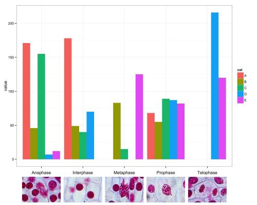
Oto jak powinno wyglądać wyjście:
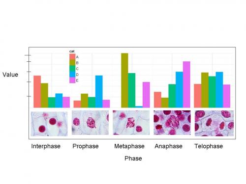
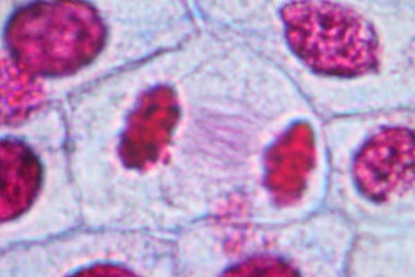
Obraz w FORMACIE jpeg może być generowany losowo (na przykładach demonstracyjnych) lub przykładowe rysunki pod linkami:
Międzyfaza prophase , metafaza, anafaza , telofaza
Edit:
Sugestia @ bapste
4 answers
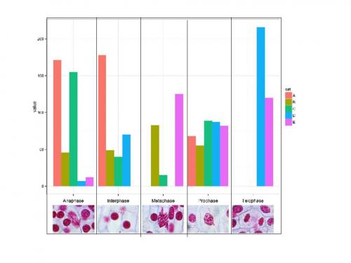
Używając pakietu grid i grając z viewportami, możesz mieć to
## transform the jpeg to raster grobs
library(jpeg)
names.axis <-  c("Interphase", "Prophase", "Metaphase", "Anaphase", "Telophase")
images <- lapply(names.axis,function(x){
  img <- readJPEG(paste('lily_',x,'.jpg',sep=''), native=TRUE)
  img <- rasterGrob(img, interpolate=TRUE)
  img
  } )
## main viewports, I divide the scene in 10 rows ans 5 columns(5 pictures)
pushViewport(plotViewport(margins = c(1,1,1,1),
             layout=grid.layout(nrow=10, ncol=5),xscale =c(1,5)))
## I put in the 1:7 rows the plot without axis
## I define my nested viewport then I plot it as a grob.
pushViewport(plotViewport(layout.pos.col=1:5, layout.pos.row=1:7,
             margins = c(1,1,1,1)))
pp <- ggplot() +
  geom_bar(data=myd, aes(y = value, x = phase, fill = cat),
                 stat="identity",position='dodge') +
  theme_bw()+theme(legend.position="none", axis.title.y=element_blank(),
                   axis.title.x=element_blank(),axis.text.x=element_blank())
gg <- ggplotGrob(pp)
grid.draw(gg)
upViewport()
## I draw my pictures in between rows 8/9 ( visual choice)
## I define a nested Viewport for each picture than I draw it.
sapply(1:5,function(x){
  pushViewport(viewport(layout.pos.col=x, layout.pos.row=8:9,just=c('top')))
  pushViewport(plotViewport(margins = c(5.2,3,4,3)))
  grid.draw(images[[x]])
  upViewport(2)
  ## I do same thing for text
  pushViewport(viewport(layout.pos.col=x, layout.pos.row=10,just=c('top')))
  pushViewport(plotViewport(margins = c(1,3,1,1)))
    grid.text(names.axis[x],gp = gpar(cex=1.5))
  upViewport(2)
})
pushViewport(plotViewport(layout.pos.col=1:5, layout.pos.row=1:9,
             margins = c(1,1,1,1)))
grid.rect(gp=gpar(fill=NA))
upViewport(2)
Warning: date(): Invalid date.timezone value 'Europe/Kyiv', we selected the timezone 'UTC' for now. in /var/www/agent_stack/data/www/doraprojects.net/template/agent.layouts/content.php on line 54
2012-12-29 15:25:48
Możesz utworzyć niestandardową funkcję elementu dla axis.text.x, ale jest to dość skomplikowane i zawiłe. Podobne wnioski zostały złożone w przeszłości, byłoby miło mieć czyste rozwiązanie dla tej i innych niestandardowych zmian (etykiety pasków, osi itp./ Align = "left" /
library(jpeg)
img <- lapply(list.files(pattern="jpg"), readJPEG )
names(img) <- c("Anaphase", "Interphase", "Metaphase", "Prophase", "Telophase")

require(ggplot2)
require(grid)

# user-level interface to the element grob
my_axis = function(img) {
    structure(
      list(img=img),
      class = c("element_custom","element_blank", "element") # inheritance test workaround
    )
  }
# returns a gTree with two children: the text label, and a rasterGrob below
element_grob.element_custom <- function(element, x,...)  {
  stopifnot(length(x) == length(element$img))
  tag <- names(element$img)
  # add vertical padding to leave space
  g1 <- textGrob(paste0(tag, "\n\n\n\n\n"), x=x,vjust=0.6)
  g2 <- mapply(rasterGrob, x=x, image = element$img[tag],
               MoreArgs = list(vjust=0.7,interpolate=FALSE,
                               height=unit(5,"lines")),
               SIMPLIFY = FALSE)

  gTree(children=do.call(gList,c(g2,list(g1))), cl = "custom_axis")
}
# gTrees don't know their size and ggplot would squash it, so give it room
grobHeight.custom_axis = heightDetails.custom_axis = function(x, ...)
  unit(6, "lines")

ggplot(myd) +
  geom_bar(aes(y = value, x = phase, fill = cat), stat="identity", position='dodge') +
  theme_bw() +
  theme(axis.text.x = my_axis(img),
          axis.title.x = element_blank())

ggsave("test.png",p,width=10,height=8)
Warning: date(): Invalid date.timezone value 'Europe/Kyiv', we selected the timezone 'UTC' for now. in /var/www/agent_stack/data/www/doraprojects.net/template/agent.layouts/content.php on line 54
2012-12-29 06:03:05
Edit: jest to uciążliwe podejście, które można łatwo złamać. Proszę rozważyć To rozwiązanie zamiast.
Oto rozwiązanie za pomocą pakietu cowplot . Niekoniecznie jest to lepsze, ponieważ wymaga trochę majstrowania przy współrzędnych, aby wszystko było prawidłowo ustawione, ale jest to alternatywa i może być bardziej elastyczna w niektórych aspektach.
# create data
set.seed(123)
myd<- expand.grid('cat' = LETTERS[1:5], 'cond'= c(F,T), 'phase' = c("Interphase", "Prophase", "Metaphase", "Anaphase", "Telophase"))
myd$value <- floor((rnorm(nrow(myd)))*100)
myd$value[myd$value < 0] <- 0

# load images
library(jpeg)
img <- lapply(list.files(pattern="jpg"), readJPEG )
names(img) <- c("Anaphase", "Interphase", "Metaphase", "Prophase", "Telophase")

# solution via cowplot, define a function that draws a strip of images
require(cowplot)
add_image_strip <- function(plot, image_list, xmin = 0, xmax = 1, y = 0, height = 1)
{
    xstep = (xmax-xmin)/length(image_list)
    for (img in image_list)
    {
        g <- grid::rasterGrob(img, interpolate=TRUE)
        plot <- plot + annotation_custom(g, xmin, xmax = xmin + xstep, ymin = y, ymax = y + height)
        xmin <- xmin + xstep
    }
    plot
}

# make the bar plot, with extra spacing at the bottom
plot.myd <- ggplot(myd) +
  geom_bar(aes(y = value, x = phase, fill = cat), stat="identity", position='dodge') +
  theme( axis.title.x = element_blank(),
         plot.margin = unit(c(1, 1, 4.5, 0.5), "lines")
        )

# place bar plot and image strip onto blanc canvas
# requires some fiddling with numbers, specific choice depends
# on `width` and `height` choices in ggsave
plot <- ggdraw(plot.myd)
plot <- add_image_strip(plot, image_list=img, xmin = .105, xmax = 0.875, y=.04, height = .18)
ggsave("test.png", plot, width=8, height=4)
Warning: date(): Invalid date.timezone value 'Europe/Kyiv', we selected the timezone 'UTC' for now. in /var/www/agent_stack/data/www/doraprojects.net/template/agent.layouts/content.php on line 54
2017-11-24 20:03:30
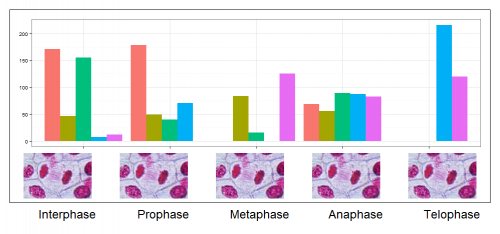
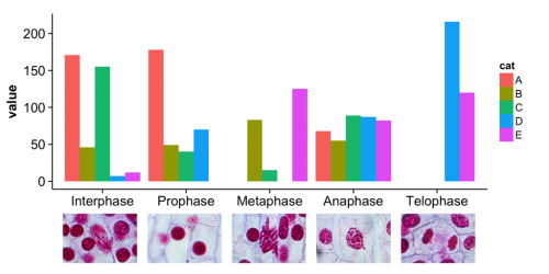
Generowanie takiej liczby stało się stosunkowo proste dzięki funkcjom dostępnym w pakiecie cowplot, w szczególności funkcjom axis_canvas() i insert_xaxis_grob(). (Zastrzeżenie: jestem autorem pakietu.)
require(cowplot)

# create the data
set.seed(123)
myd <- expand.grid('cat' = LETTERS[1:5], 'cond'= c(F,T), 'phase' = c("Interphase", "Prophase", "Metaphase", "Anaphase", "Telophase"))
myd$value <- floor((rnorm(nrow(myd)))*100)
myd$value[myd$value < 0] <- 0

# make the barplot
pbar <- ggplot(myd) +
  geom_bar(aes(y = value, x = phase, fill = cat), stat="identity", position='dodge') +
  scale_y_continuous(limits = c(0, 224), expand = c(0, 0)) +
  theme_minimal(14) +
  theme(axis.ticks.length = unit(0, "in"))

# make the image strip
pimage <- axis_canvas(pbar, axis = 'x') +
  draw_image("http://www.microbehunter.com/wp/wp-content/uploads/2009/lily_interphase.jpg", x = 0.5, scale = 0.9) +
  draw_image("http://www.microbehunter.com/wp/wp-content/uploads/2009/lily_prophase.jpg", x = 1.5, scale = 0.9) +
  draw_image("http://www.microbehunter.com/wp/wp-content/uploads/2009/lily_metaphase2.jpg", x = 2.5, scale = 0.9) +
  draw_image("http://www.microbehunter.com/wp/wp-content/uploads/2009/lily_anaphase2.jpg", x = 3.5, scale = 0.9) +
  draw_image("http://www.microbehunter.com/wp/wp-content/uploads/2009/lily_telophase.jpg", x = 4.5, scale = 0.9)

# insert the image strip into the bar plot and draw
ggdraw(insert_xaxis_grob(pbar, pimage, position = "bottom"))

Czytam obrazy prosto z sieci, ale funkcja draw_image() będzie działać również z plikami lokalnymi.
Teoretycznie powinno być możliwe narysowanie paska obrazu za pomocą geom_image() z pakietu ggimage, ale nie mogłem go uruchomić bez miałem zniekształcone obrazy, więc uciekłem się do pięciu połączeń.
Warning: date(): Invalid date.timezone value 'Europe/Kyiv', we selected the timezone 'UTC' for now. in /var/www/agent_stack/data/www/doraprojects.net/template/agent.layouts/content.php on line 54
2017-11-24 20:46:17