Cieniowanie wykresu gęstości jądra między dwoma punktami.
Często używam Wykresów gęstości jądra do zilustrowania dystrybucji. Są one łatwe i szybkie do utworzenia w R jak tak:
set.seed(1)
draws <- rnorm(100)^2
dens <- density(draws)
plot(dens)
#or in one line like this: plot(density(rnorm(100)^2))
Co daje mi ten ładny mały PDF:

quantile:
q75 <- quantile(draws, .75)
q95 <- quantile(draws, .95)
Ale jak zacienić obszar pomiędzy q75 i q95?
5 answers
Z funkcją polygon(), zobacz jej stronę pomocy i sądzę, że mieliśmy podobne pytania również tutaj.
Musisz znaleźć indeks wartości kwantyli, aby uzyskać rzeczywiste pary (x,y).
Edit: proszę bardzo:
x1 <- min(which(dens$x >= q75))
x2 <- max(which(dens$x <  q95))
with(dens, polygon(x=c(x[c(x1,x1:x2,x2)]), y= c(0, y[x1:x2], 0), col="gray"))
Output (dodany przez JDL)

Warning: date(): Invalid date.timezone value 'Europe/Kyiv', we selected the timezone 'UTC' for now. in /var/www/agent_stack/data/www/doraprojects.net/template/agent.layouts/content.php on line 54
2017-05-01 10:34:46
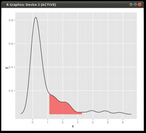
Inne rozwiązanie:
dd <- with(dens,data.frame(x,y))
library(ggplot2)
qplot(x,y,data=dd,geom="line")+
  geom_ribbon(data=subset(dd,x>q75 & x<q95),aes(ymax=y),ymin=0,
              fill="red",colour=NA,alpha=0.5)
Wynik:
Warning: date(): Invalid date.timezone value 'Europe/Kyiv', we selected the timezone 'UTC' for now. in /var/www/agent_stack/data/www/doraprojects.net/template/agent.layouts/content.php on line 54
2010-12-07 04:34:01
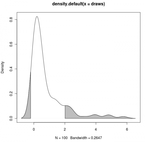
Rozwiązanie rozszerzone:
Jeśli chcesz przyciemnić oba ogony (skopiuj i wklej kod Dirka) i użyć znanych wartości x:
set.seed(1)
draws <- rnorm(100)^2
dens <- density(draws)
plot(dens)

q2     <- 2
q65    <- 6.5
qn08   <- -0.8
qn02   <- -0.2

x1 <- min(which(dens$x >= q2))
x2 <- max(which(dens$x <  q65))
x3 <- min(which(dens$x >= qn08))
x4 <- max(which(dens$x <  qn02))

with(dens, polygon(x=c(x[c(x1,x1:x2,x2)]), y= c(0, y[x1:x2], 0), col="gray"))
with(dens, polygon(x=c(x[c(x3,x3:x4,x4)]), y= c(0, y[x3:x4], 0), col="gray"))
Wynik:
Warning: date(): Invalid date.timezone value 'Europe/Kyiv', we selected the timezone 'UTC' for now. in /var/www/agent_stack/data/www/doraprojects.net/template/agent.layouts/content.php on line 54
2015-06-21 21:36:56
To pytanie wymaga odpowiedzi. Oto bardzo podstawowy, po prostu dostosowując metodę zastosowaną przez Dirka i innych: {]}
#Set up the data
set.seed(1)
draws <- rnorm(100)^2
dens <- density(draws)

#Put in a simple data frame
d <- data.frame(x = dens$x, y = dens$y)

#Define a custom panel function;
# Options like color don't need to be hard coded
shadePanel <- function(x,y,shadeLims){
    panel.lines(x,y)
    m1 <- min(which(x >= shadeLims[1]))
    m2 <- max(which(x <= shadeLims[2]))
    tmp <- data.frame(x1 = x[c(m1,m1:m2,m2)], y1 = c(0,y[m1:m2],0))
    panel.polygon(tmp$x1,tmp$y1,col = "blue")
}

#Plot
xyplot(y~x,data = d, panel = shadePanel, shadeLims = c(1,3))
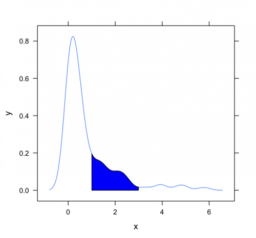
Warning: date(): Invalid date.timezone value 'Europe/Kyiv', we selected the timezone 'UTC' for now. in /var/www/agent_stack/data/www/doraprojects.net/template/agent.layouts/content.php on line 54
2011-08-25 02:48:07
Oto kolejny wariant ggplot2 oparty na funkcji przybliżającej gęstość jądra przy oryginalnych wartościach danych:
approxdens <- function(x) {
    dens <- density(x)
    f <- with(dens, approxfun(x, y))
    f(x)
}

Korzystanie z oryginalnych danych (zamiast tworzenia nowej ramki danych z wartości X i y oszacowania gęstości) ma tę zaletę, że działa również w powierzchownych Wykresów, gdzie wartości kwantyl zależy od zmiennej, w której dane są zgrupowane:

Użyty kod
library(tidyverse)
library(RColorBrewer)

# dummy data
set.seed(1)
n <- 1e2
dt <- tibble(value = rnorm(n)^2)

# function that approximates the density at the provided values
approxdens <- function(x) {
    dens <- density(x)
    f <- with(dens, approxfun(x, y))
    f(x)
}

probs <- c(0.75, 0.95)

dt <- dt %>%
    mutate(dy = approxdens(value),                         # calculate density
           p = percent_rank(value),                        # percentile rank
           pcat = as.factor(cut(p, breaks = probs,         # percentile category based on probs
                                include.lowest = TRUE)))

ggplot(dt, aes(value, dy)) +
    geom_ribbon(aes(ymin = 0, ymax = dy, fill = pcat)) +
    geom_line() +
    scale_fill_brewer(guide = "none") +
    theme_bw()


# dummy data with 2 groups
dt2 <- tibble(category = c(rep("A", n), rep("B", n)),
              value = c(rnorm(n)^2, rnorm(n, mean = 2)))

dt2 <- dt2 %>%
    group_by(category) %>%
    mutate(dy = approxdens(value),
           p = percent_rank(value),
           pcat = as.factor(cut(p, breaks = probs,
                                include.lowest = TRUE)))

# faceted plot
ggplot(dt2, aes(value, dy)) +
    geom_ribbon(aes(ymin = 0, ymax = dy, fill = pcat)) +
    geom_line() +
    facet_wrap(~ category, nrow = 2, scales = "fixed") +
    scale_fill_brewer(guide = "none") +
    theme_bw()
Warning: date(): Invalid date.timezone value 'Europe/Kyiv', we selected the timezone 'UTC' for now. in /var/www/agent_stack/data/www/doraprojects.net/template/agent.layouts/content.php on line 54
2018-07-13 18:23:58