Jak narysować dwa histogramy razem w R?
Używam R i mam dwie ramki danych: marchew i ogórek. Każda ramka danych ma pojedynczą kolumnę liczbową, która wyświetla długość wszystkich mierzonych marchwi (łącznie: 100k marchwi) i ogórków (łącznie: 50k ogórków).
Chciałbym narysować dwa histogramy-długość marchwi i długość ogórków-na tej samej działce. Nakładają się na siebie, więc chyba też potrzebuję przejrzystości. Muszę również użyć częstotliwości względnych, a nie liczb bezwzględnych, ponieważ liczba instancji w każdej grupie jest inna.
Coś takiego byłoby fajne ale nie rozumiem jak to stworzyć z moich dwóch tabel:
8 answers
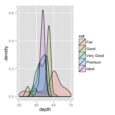
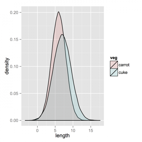
Obraz, z którym się połączyłeś, był dla krzywych gęstości, a nie histogramów.
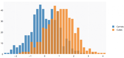
Jeśli czytałeś na ggplot to może jedyne, czego ci brakuje, to połączenie dwóch ramek danych w jedną długą.
Zacznijmy więc od czegoś takiego jak to, co masz, dwa oddzielne zestawy danych i połącz je.
carrots <- data.frame(length = rnorm(100000, 6, 2))
cukes <- data.frame(length = rnorm(50000, 7, 2.5))

#Now, combine your two dataframes into one.  First make a new column in each that will be a variable to identify where they came from later.
carrots$veg <- 'carrot'
cukes$veg <- 'cuke'

#and combine into your new data frame vegLengths
vegLengths <- rbind(carrots, cukes)
Po tym, co jest niepotrzebne, jeśli Twoje dane są już długie, potrzebujesz tylko jednej linii, aby stworzyć swój wykres.
ggplot(vegLengths, aes(length, fill = veg)) + geom_density(alpha = 0.2)
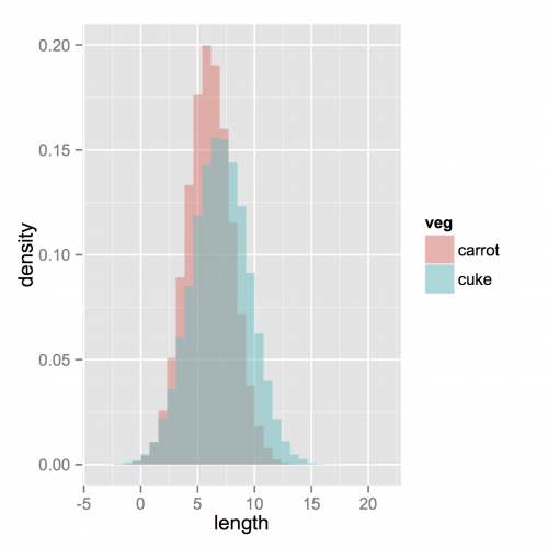
Teraz, jeśli naprawdę chciałem histogramy, które będą działać. Zauważ, że musisz zmienić pozycję z domyślnego argumentu "stos". Możesz to przegapić, jeśli tak naprawdę nie masz pojęcia, jak powinny wyglądać Twoje dane. Wyższa Alfa wygląda tam lepiej. Zauważ również, że zrobiłem to histogramy gęstości. Łatwo jest usunąć y = ..density.., aby wrócić do liczenia.
ggplot(vegLengths, aes(length, fill = veg)) + geom_histogram(alpha = 0.5, aes(y = ..density..), position = 'identity')
Warning: date(): Invalid date.timezone value 'Europe/Kyiv', we selected the timezone 'UTC' for now. in /var/www/agent_stack/data/www/doraprojects.net/template/agent.layouts/content.php on line 54
2017-06-20 05:37:36
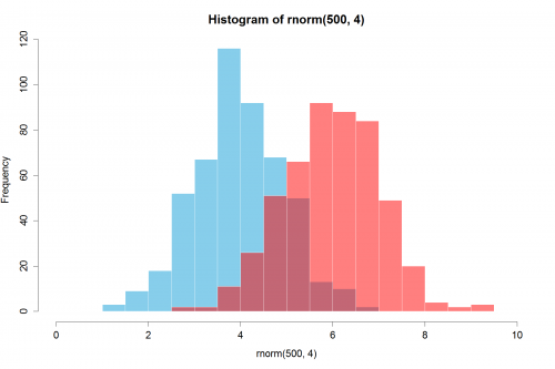
Oto jeszcze prostsze rozwiązanie wykorzystujące grafikę podstawową i mieszanie alfa (które nie działa na wszystkich urządzeniach graficznych):
set.seed(42)
p1 <- hist(rnorm(500,4))                     # centered at 4
p2 <- hist(rnorm(500,6))                     # centered at 6
plot( p1, col=rgb(0,0,1,1/4), xlim=c(0,10))  # first histogram
plot( p2, col=rgb(1,0,0,1/4), xlim=c(0,10), add=T)  # second
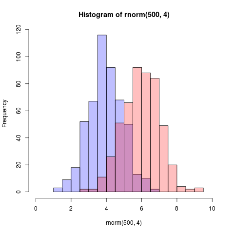
Edit, ponad dwa lata później: jako że to właśnie się poprawiło, równie dobrze mogę dodać wizualizację tego, co Kod produkuje jako alpha-blending jest tak cholernie przydatny:
Warning: date(): Invalid date.timezone value 'Europe/Kyiv', we selected the timezone 'UTC' for now. in /var/www/agent_stack/data/www/doraprojects.net/template/agent.layouts/content.php on line 54
2012-09-21 01:36:46
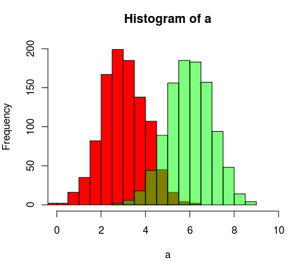
Oto funkcja, którą napisałem, że używa pseudo-przezroczystości do reprezentowania nakładających się histogramów
plotOverlappingHist <- function(a, b, colors=c("white","gray20","gray50"),
                                breaks=NULL, xlim=NULL, ylim=NULL){

  ahist=NULL
  bhist=NULL

  if(!(is.null(breaks))){
    ahist=hist(a,breaks=breaks,plot=F)
    bhist=hist(b,breaks=breaks,plot=F)
  } else {
    ahist=hist(a,plot=F)
    bhist=hist(b,plot=F)

    dist = ahist$breaks[2]-ahist$breaks[1]
    breaks = seq(min(ahist$breaks,bhist$breaks),max(ahist$breaks,bhist$breaks),dist)

    ahist=hist(a,breaks=breaks,plot=F)
    bhist=hist(b,breaks=breaks,plot=F)
  }

  if(is.null(xlim)){
    xlim = c(min(ahist$breaks,bhist$breaks),max(ahist$breaks,bhist$breaks))
  }

  if(is.null(ylim)){
    ylim = c(0,max(ahist$counts,bhist$counts))
  }

  overlap = ahist
  for(i in 1:length(overlap$counts)){
    if(ahist$counts[i] > 0 & bhist$counts[i] > 0){
      overlap$counts[i] = min(ahist$counts[i],bhist$counts[i])
    } else {
      overlap$counts[i] = 0
    }
  }

  plot(ahist, xlim=xlim, ylim=ylim, col=colors[1])
  plot(bhist, xlim=xlim, ylim=ylim, col=colors[2], add=T)
  plot(overlap, xlim=xlim, ylim=ylim, col=colors[3], add=T)
}
Oto inny sposób, aby to zrobić, używając obsługi R dla przezroczystych kolorów
a=rnorm(1000, 3, 1)
b=rnorm(1000, 6, 1)
hist(a, xlim=c(0,10), col="red")
hist(b, add=T, col=rgb(0, 1, 0, 0.5) )
Wyniki wyglądają tak:
Warning: date(): Invalid date.timezone value 'Europe/Kyiv', we selected the timezone 'UTC' for now. in /var/www/agent_stack/data/www/doraprojects.net/template/agent.layouts/content.php on line 54
2013-07-05 01:59:16
Już są piękne odpowiedzi, ale pomyślałem o dodaniu tego. Dla mnie wygląda dobrze.
(Skopiowane liczby losowe z @ Dirk). library(scales) is needed "
set.seed(42)
hist(rnorm(500,4),xlim=c(0,10),col='skyblue',border=F)
hist(rnorm(500,6),add=T,col=scales::alpha('red',.5),border=F)
Wynik jest...
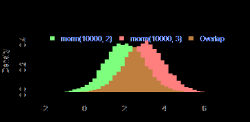
Update: ta nakładająca się funkcja może być również przydatna dla niektórych.
hist0 <- function(...,col='skyblue',border=T) hist(...,col=col,border=border)
Czuję, że wynik z hist0 jest ładniejszy niż hist
hist2 <- function(var1, var2,name1='',name2='',
              breaks = min(max(length(var1), length(var2)),20),
              main0 = "", alpha0 = 0.5,grey=0,border=F,...) {

library(scales)
  colh <- c(rgb(0, 1, 0, alpha0), rgb(1, 0, 0, alpha0))
  if(grey) colh <- c(alpha(grey(0.1,alpha0)), alpha(grey(0.9,alpha0)))

  max0 = max(var1, var2)
  min0 = min(var1, var2)

  den1_max <- hist(var1, breaks = breaks, plot = F)$density %>% max
  den2_max <- hist(var2, breaks = breaks, plot = F)$density %>% max
  den_max <- max(den2_max, den1_max)*1.2
  var1 %>% hist0(xlim = c(min0 , max0) , breaks = breaks,
                 freq = F, col = colh[1], ylim = c(0, den_max), main = main0,border=border,...)
  var2 %>% hist0(xlim = c(min0 , max0),  breaks = breaks,
                 freq = F, col = colh[2], ylim = c(0, den_max), add = T,border=border,...)
  legend(min0,den_max, legend = c(
    ifelse(nchar(name1)==0,substitute(var1) %>% deparse,name1),
    ifelse(nchar(name2)==0,substitute(var2) %>% deparse,name2),
    "Overlap"), fill = c('white','white', colh[1]), bty = "n", cex=1,ncol=3)

  legend(min0,den_max, legend = c(
    ifelse(nchar(name1)==0,substitute(var1) %>% deparse,name1),
    ifelse(nchar(name2)==0,substitute(var2) %>% deparse,name2),
    "Overlap"), fill = c(colh, colh[2]), bty = "n", cex=1,ncol=3) }
Wynik
par(mar=c(3, 4, 3, 2) + 0.1)
set.seed(100)
hist2(rnorm(10000,2),rnorm(10000,3),breaks = 50)
Jest
Warning: date(): Invalid date.timezone value 'Europe/Kyiv', we selected the timezone 'UTC' for now. in /var/www/agent_stack/data/www/doraprojects.net/template/agent.layouts/content.php on line 54
2015-12-03 19:20:08
Oto przykład jak można to zrobić w "klasycznej" grafice R:
## generate some random data
carrotLengths <- rnorm(1000,15,5)
cucumberLengths <- rnorm(200,20,7)
## calculate the histograms - don't plot yet
histCarrot <- hist(carrotLengths,plot = FALSE)
histCucumber <- hist(cucumberLengths,plot = FALSE)
## calculate the range of the graph
xlim <- range(histCucumber$breaks,histCarrot$breaks)
ylim <- range(0,histCucumber$density,
              histCarrot$density)
## plot the first graph
plot(histCarrot,xlim = xlim, ylim = ylim,
     col = rgb(1,0,0,0.4),xlab = 'Lengths',
     freq = FALSE, ## relative, not absolute frequency
     main = 'Distribution of carrots and cucumbers')
## plot the second graph on top of this
opar <- par(new = FALSE)
plot(histCucumber,xlim = xlim, ylim = ylim,
     xaxt = 'n', yaxt = 'n', ## don't add axes
     col = rgb(0,0,1,0.4), add = TRUE,
     freq = FALSE) ## relative, not absolute frequency
## add a legend in the corner
legend('topleft',c('Carrots','Cucumbers'),
       fill = rgb(1:0,0,0:1,0.4), bty = 'n',
       border = NA)
par(opar)
Jedyny problem z tym polega na tym, że wygląda to znacznie lepiej, jeśli przerwy histogramu są wyrównane, co może być wykonane ręcznie(w argumentach przekazanych do hist).
Warning: date(): Invalid date.timezone value 'Europe/Kyiv', we selected the timezone 'UTC' for now. in /var/www/agent_stack/data/www/doraprojects.net/template/agent.layouts/content.php on line 54
2015-01-28 02:42:58
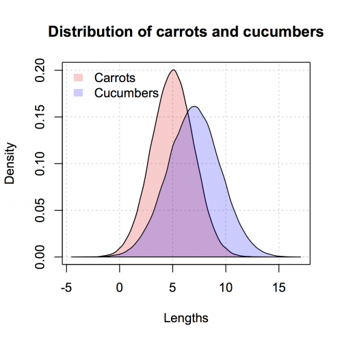
Oto wersja podobna do ggplot2, którą dałem tylko w base R. skopiowałem trochę z @nullglob.
Wygeneruj DANE
carrots <- rnorm(100000,5,2)
cukes <- rnorm(50000,7,2.5)
Nie musisz umieszczać go w ramce danych, jak w przypadku ggplot2. Wadą tej metody jest to, że trzeba napisać o wiele więcej szczegółów fabuły. Zaletą jest to, że masz kontrolę nad większą ilością szczegółów działki.
## calculate the density - don't plot yet
densCarrot <- density(carrots)
densCuke <- density(cukes)
## calculate the range of the graph
xlim <- range(densCuke$x,densCarrot$x)
ylim <- range(0,densCuke$y, densCarrot$y)
#pick the colours
carrotCol <- rgb(1,0,0,0.2)
cukeCol <- rgb(0,0,1,0.2)
## plot the carrots and set up most of the plot parameters
plot(densCarrot, xlim = xlim, ylim = ylim, xlab = 'Lengths',
     main = 'Distribution of carrots and cucumbers',
     panel.first = grid())
#put our density plots in
polygon(densCarrot, density = -1, col = carrotCol)
polygon(densCuke, density = -1, col = cukeCol)
## add a legend in the corner
legend('topleft',c('Carrots','Cucumbers'),
       fill = c(carrotCol, cukeCol), bty = 'n',
       border = NA)
Warning: date(): Invalid date.timezone value 'Europe/Kyiv', we selected the timezone 'UTC' for now. in /var/www/agent_stack/data/www/doraprojects.net/template/agent.layouts/content.php on line 54
2013-10-15 01:56:27
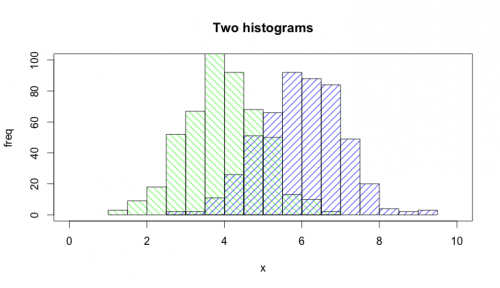
@Dirk Eddelbuettel: podstawowa idea jest doskonała, ale Kod, jak pokazano, można poprawić. [Długo trwa Wyjaśnienie, stąd osobna odpowiedź, a nie komentarz.]
Funkcja hist() domyślnie rysuje wykresy, więc musisz dodać opcję plot=FALSE. Co więcej, jaśniejsze jest określenie obszaru wykresu za pomocą wywołania plot(0,0,type="n",...), w którym można dodać etykiety osi, tytuł wykresu itp. Na koniec chciałbym wspomnieć, że można również użyć cieniowania, aby odróżnić dwa histogramy. Oto kod:
set.seed(42)
p1 <- hist(rnorm(500,4),plot=FALSE)
p2 <- hist(rnorm(500,6),plot=FALSE)
plot(0,0,type="n",xlim=c(0,10),ylim=c(0,100),xlab="x",ylab="freq",main="Two histograms")
plot(p1,col="green",density=10,angle=135,add=TRUE)
plot(p2,col="blue",density=10,angle=45,add=TRUE)
A oto wynik (trochę za szeroki ze względu na RStudio : -)):
Warning: date(): Invalid date.timezone value 'Europe/Kyiv', we selected the timezone 'UTC' for now. in /var/www/agent_stack/data/www/doraprojects.net/template/agent.layouts/content.php on line 54
2014-10-09 15:18:43
API R Plotly ' ego może być dla Ciebie przydatne. Poniższy wykres jest tutaj .
library(plotly)
#add username and key
p <- plotly(username="Username", key="API_KEY")
#generate data
x0 = rnorm(500)
x1 = rnorm(500)+1
#arrange your graph
data0 = list(x=x0,
         name = "Carrots",
         type='histogramx',
         opacity = 0.8)

data1 = list(x=x1,
         name = "Cukes",
         type='histogramx',
         opacity = 0.8)
#specify type as 'overlay'
layout <- list(barmode='overlay',
               plot_bgcolor = 'rgba(249,249,251,.85)')
#format response, and use 'browseURL' to open graph tab in your browser.
response = p$plotly(data0, data1, kwargs=list(layout=layout))

url = response$url
filename = response$filename

browseURL(response$url)
Warning: date(): Invalid date.timezone value 'Europe/Kyiv', we selected the timezone 'UTC' for now. in /var/www/agent_stack/data/www/doraprojects.net/template/agent.layouts/content.php on line 54
2014-03-26 05:25:29